Guide to building a Capacity Model – Part 3

Full series: capacity modelling guide

Part 2 of this series discussed how a forecast of component usage could be calculated; using the situation where no business forecast data was available. In this penultimate part, we will look at how user-driven scenarios can be built, to provide flexibility in the model. This may not be of paramount importance to all of you; you may just want to develop a capacity forecast, which was covered in the last two blogs of the series. But, if you expect the model to be used by others, you should consider the controls and aesthetics that you can provide to the users.

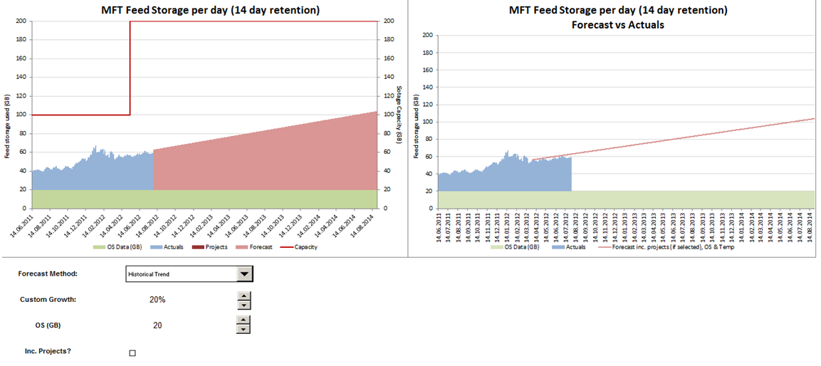
For ease of explanation, I have included the output of the capacity model below (the charts and controls below were all arrange on a single worksheet). I will then explain various steps to generating this output.

Forecast Method

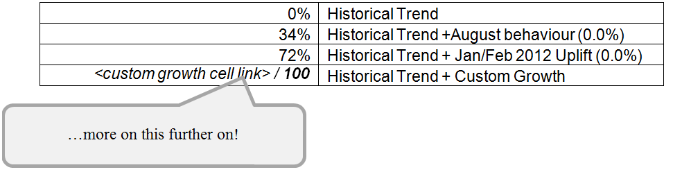
As we do not have business forecasts, I wanted to allow users to inflate the resource to allow various scenarios to be modelled. However, I also wanted to provide some information about the levels of growth that have been experienced historically. After discussions with the business, I discovered that there were two key periods when major releases took place. I analysed the file storage space used during these periods and compared it to the rest of the data, to calculate a percentage uplift that represented these events. I documented these in a table on the admin sheet.

Next, I needed to give the user a way of selecting one of the forecast methods. This can be done in two steps:

1. Select a cell on the admin sheet to be used to store the user’s chosen forecast method and name it accordingly
2. Select the Developer Tab and then Insert > Combo Box (you may need to add the Developer tab to your Microsoft Excel ribbon if it’s not there by default). There are two types of each control available in Microsoft Excel; Form and ActiveX. A simple Google search will explain the pros and cons of each; I have used a Form control in this example as I do not need any complex functionality.

Once you have added the Combo Box to the output sheet, right-click and select Format Control to adjust its settings:

• Input Range: these are the options that you want to appear in the combo box (this is the second column in the table above)
• Cell Link: this is the cell that will store the current combo box selection, created in step 1 above
• Drop down lines: this is the number of lines to appear when the combo box is selected.

Next, you need your forecast to adjust based on the chosen forecast method. Currently, our forecast calculation is as follows:

( x SLOPE) + INTERCEPT  

The cell link created in step 1 above will store an index to the user’s selection from the input range.  So, if the user has selected the “Historical Trend” forecast method, the named cell will contain a 1. Therefore, we can use the index position to pick up the corresponding percentage uplift from the table as follows:

OFFSET(

This will pick up the right percentage uplift based on the chosen forecast method. We can then apply this to our current forecast value. The resultant formula for the forecast is therefore:

(( x SLOPE) + INTERCEPT) x (1+ OFFSET(

Custom Growth

If the user selects the fourth Forecast Method, we want them to be able to specify the amount of growth they’d like to add to the forecast. This is done using a Spin Button,   which operates in the same way as the Combo Box described in the Forecast Method section above:

The following controls need to be set on the Spin Button:

• Maximum Value: to ensure that the custom growth cannot grow beyond a certain percentage (I have chosen 500%)
• Incremental Change: to determine the change you want to apply each time the spin button is used. I have used 10% in my example
• Cell Link: this a cell that I will use to store the value of the spin button. In this case, it should be somewhere on the admin sheet as it needs to be formatted into a percentage before being displayed to the user. The cell that the spin button is linked to can be named appropriately.

To display the correct custom percentage on the output sheet, use the formula

/ 100  

and then format the cell as a percentage. This same formula should be used in the table on the admin sheet which contains the four Forecast Methods. You now have a parameter to add a custom uplift to the forecast storage size. This should automatically apply to the forecast value whenever the spin button is changed.

OS Data

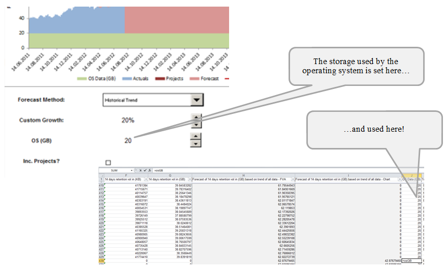
The resource data that we used in our forecast was calculated based on the volume of files loaded into the database per day. These daily volumes were summed over every 14 day period to determine the file storage space used. In this particular example, the disk being capacity modelled also needed storage space for the operating system. This usage should remain fairly constant over time. For extra flexibility, we have parameterised this value so that the user can easily change the amount of storage used by the operating system and see the effect on overall storage capacity. This is also achieved using a Spin Button

The following controls needs to be set on the Spin Button:

• Maximum Value: to ensure that the OS storage usage cannot grow uncontrollably
• Incremental Change: to determine the change you want to apply each time the spin button is used. I have used 5 GB in my example
• Cell Link: this is the cell that will be used to store the value of the spin button, which is the amount of storage used by the OS in this example. For this parameter we can refer to a cell link on the output sheet, as we do not need to format this value in any way.

You should now have a spin button that changes the amount of storage used by the operating system and updates the appropriate cell. As you have given this cell a name, you can now set the value in a new column in your data sheet, to refer to this name. This means that for every data point you have an OS size value too.

That concludes this part of the blog series. At this point, we have built some flexibility into the model to allow the user to easily consider various scenarios. In the next and final part we will look at incorporating project growth into the model and some tweaks to build our required charts.

Full series: capacity modelling guide